Are We Facing a Global “Lost Decade?”

By Steve Keen, Head Of School Of Economics, History & Politics, Kingston University

The era of low growth known as Japan’s “Lost Decade” commenced in 1990, and persists to this day.  While most authors acknowledge that the seeds for the Lost Decade were sown by excessive credit growth in the preceding Bubble Economy years, only Richard Koo (Koo, 2009, Koo, 2011, Koo, 2003, Koo, 2014) and Richard Werner (Voutsinas and Werner, 2011, Werner, 2002) have systematically argued that insufficient credit growth during the “Lost Decade” explains Japan’s now quarter-century long slump. Yet these arguments tell us more about the dilemmas facing today’s world economy than many more commonly accepted explanations of the current slowdown.

The insufficient credit growth story is rejected out of hand by most economists, for reasons summed up by Paul Krugman. From the perspective of mainstream economics, any event that negatively affects debtors is, to a large degree, offset by the positive effects of that event for creditors. Krugman therefore sees no possibility of Koo’s argument of “an entire economy being “balance-sheet constrained”:Maybe part of the problem is that Koo envisages an economy in which everyone is balance-sheet constrained, as opposed to one in which lots of people are balance-sheet constrained. I’d say that his vision makes no sense: where there are debtors, there must also be creditors, so there have to be at least some people who can respond to lower real interest rates even in a balance-sheet recession. (Krugman, 2013)

Koo is, however, correct: it is possible for an entire economy to be balance-sheet constrained. Understanding why requires an appreciation of private credit creation that goes beyond the mere accounting truism that every entity’s liability is another entity’s asset. This paper will argue that the assumptions made by mainstream economists about the role of credit and banking in the economy are incorrect. When taking into account the “money creation” functions of banking, it becomes clear that the USA and most advanced economies as well as many emerging economies have joined Japan in being balance-sheet constrained, and face their own “lost decade” as a consequence of low credit growth.

I will start with the empirical data and its implications, and then move on to  the argument that an entire economy can be balance-sheet constrained.[1]

The Empirical Data

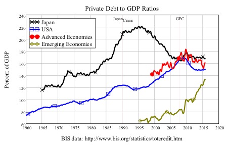
Japan’s private debt to GDP ratio was once in a league of its own—reflecting the Keiretsu system of industry being financed by affiliated banks. At 115% of GDP, Japan’s private debt to GDP ratio was 1.3 times the USA’s 86% ratio in 1965, and the ratio rose to 1.67 times by the start of the “Lost Decade.”[2] However, from then until the start of the US crisis (the “Global Financial Crisis” or “GFC”) in August 2007, the growth of Japan’s debt to GDP ratio slowed down dramatically. The ratio peaked at 220% in 1995, and then fell while the US ratio continued to rise during the Internet and Subprime bubbles. When the GFC began, the USA and Japan were tied, with private debt ratios of 165% of GDP (see Figure 1).  In the aftermath to the GFC, Japan’s private debt ratio has stabilized at roughly 170% of GDP, which now puts it 10% above the advanced economy average, and 20% above the USA’s current level of 150% of GDP.

Figure 1: Japan’s private debt ratio was higher than the USA’s until the 2008 crisis

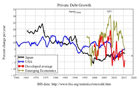
While Japan’s private debt to GDP ratio was exceptional, the growth rate of credit in Japan prior to its crisis was less so: though it had the highest growth rate in the pre-1990 era (at almost 25% p.a. in 1973), from 1975 onwards its growth of credit per year was normally in the middle of the advanced economies pack. The average growth of private debt from 1966 till 1990 in Japan was 12% per year, versus 9.5% for the USA and 13.5% per year for the 14 countries for which the BIS has data.[3]

This changed dramatically after its crisis at the end of 1990: from the end of 1991 on, the rate of growth of private credit in Japan dropped to minus 0.5% per year on average, while credit in the USA grew at the slower but still substantial rate of 6.5% per year. After the financial crisis of 2007-8, the growth rate of private debt in the USA turned negative for the first time since the Great Depression, falling by as much as 5% of GDP in 2010.  Credit growth resumed in the USA in 2011, but on average, since 2008, the growth rate is an anemic 1.8% per year (see Figure 2).

Figure 2: Private credit growth per year

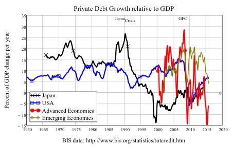
As Figure 3 shows, the fact that private debt rose faster than GDP prior to both Japan’s and the USA’s crises means that the relative importance of a change in credit has risen over time. Since Japan’s private debt to GDP ratio has been above 100% since records began, the change in credit measured as a percentage of GDP has always been a greater magnitude than the percentage change in credit itself. Thus credit growth averaged 17% of GDP per year in Japan before its crisis, 1% between its crisis and the financial crisis of 2007-8, and minus 0.66% of GDP per year since the financial crisis. The comparable figures for the USA are 9.5% of GDP per year from 1965 till Japan’s crisis (over which time, the USA’s private debt to GDP ratio rose from 80% to 120%), 9% between Japan’s crisis and the GFC, and 2.8% of GDP per year since the GFC.

Figure 3: Credit growth shown as a percentage of GDP

The “balance sheet constrained” analysis argues that a slowdown in the rate of growth of credit will cause a reduction in aggregate demand and income, and therefore lower growth in our demand-led economies. Since Japan reached the balance sheet constrained state roughly 18 years before the rest of the OECD, this analysis implies that Japan’s low to negative credit-growth (and resulting tardy economic growth) is a taste of what the USA and most of the rest of the global economy can expect if they are as ineffective at tackling the real cause of the crisis as Japan itself has been.

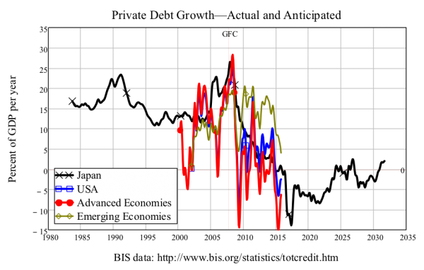
Figure 4 gives a picture of what that future might bring: an average change in credit that is substantially negative, so that the change in credit subtracts from demand rather than adding to it. While Japan’s private sector debt performance reflects a huge offsetting increase in public debt—which, for both political and current account reasons, is unlikely to be replicated in other nations—the implication one can extrapolate for the world in general from Japan’s last two decades is that the era of credit-led growth is over, and economic growth will stagnate as a result.

Figure 4: What credit growth could look like for the next 20 years given Japan’s experience since 1990

Credit growth, money creation and aggregate demand

The above analysis is dismissed by mainstream economists on the basis of a model of money and banking—known as “Loanable Funds”—that denies any key role in macroeconomics for the aggregate level of debt. According to this theory, lending represents no more than a redistribution of existing spending power between different agents: it does not create any additional spending power in its own right. Bernanke used this argument to dismiss Fisher’s “Debt Deflation” explanation for the Great Depression:Fisher’s idea was less influential in academic circles, though, because of the counterargument that debt-deflation represented no more than a redistribution from one group (debtors) to another (creditors). Absent implausibly large differences in marginal spending propensities among the groups, it was suggested, pure redistributions should have no significant macro-economic effects. (Bernanke, 2000, p. 24)

The key characteristic of “Loanable Funds” is that it treats a bank only as an “intermediary” between savers and investors, rather than as a loan originator in its own right. Since such a loan transfers an amount of money from the saver’s account to the investor’s, no additional money is created, and the rise in the investor’s spending power is at least partially offset by the decline in the saver’s (and vice-versa when debt is repaid). There is, therefore, no link between changes in the level of debt and changes in the money supply in this model, as Krugman emphasizes:Think of it this way: when debt is rising, it’s not the economy as a whole borrowing more money. It is, rather, a case of less patient people—people who for whatever reason want to spend sooner rather than later—borrowing from more patient people. (Krugman, 2012, pp. 146-147)

Krugman’s assertion that there is no link between rising debt and a rising money supply raises the issue of what the money supply is. As the Bank of England observes, “most money takes the form of bank deposits” (McLeay et al., 2014, p. 14), with notes and coins—which today are created only by the government–making up the remainder. In contrast to Krugman, the Bank of England argues that banks do originate loans, and that this is economically significant, since when they do, the increase in debt causes an equivalent increase in the money supply:

The reality of how money is created today differs from the description found in some economics textbooks:

• Rather than banks receiving deposits when households save and then lending them out, bank lending creates deposits.
• In normal times, the central bank does not fix the amount of money in circulation, nor is central bank money ‘multiplied up’ into more loans and deposits…
• Whenever a bank makes a loan, it simultaneously creates a matching deposit in the borrower’s bank account, thereby creating new money. (McLeay et al., 2014, p. 14)[4]

In making this argument, the Bank of England has supported a long line of non-mainstream economists who have argued that bank lending creates money (Fontana and Realfonzo, 2005, Graziani, 1989, Minsky, 1980, Moore, 1979, Wray, 1989, Bell, 1998).[5]

I argue that, as well as creating money, when the money brought into existence by a bank loan is spent, an equivalent increase in aggregate demand (and either aggregate income or aggregate capital gains) occurs as well.    (See the Appendix for the formal proof).

Most loans are effectively “spent into existence”: after a loan is approved (say for a mortgage), so no debt liability is incurred by the borrower until the borrowed money is transferred to the seller. Thus the loan and the expenditure financed by the loan appear simultaneously, and the expenditure of the loan becomes income (or a source of capital gain) for the seller. This is the macroeconomic reason that bank debt matters: the change in bank debt is a major—and by far the most volatile—source of aggregate demand. This does not happen in the Loanable Funds model, which is why it is a wildly misleading guide to macroeconomic policy.

This difference between these two models—the unrealistic “Loanable Funds” model used by conventional economists, and the realistic “Endogenous Money” model developed by Post Keynesian economists and now supported by the Bank of England—can be seen by contrasting the next two tables.

In Loanable Funds, the act of lending redistributes money from the Saver to the Borrower—there is no new money creation (Table 1). When the borrowed money is spent, the Borrower ends up with the purchased goods or assets, no change in its deposit account, and a debt to the Saver (which does not appear on the Bank’s ledger, since the debt is neither an asset nor a liability of the Bank itself). There is no change in the aggregate amount of money, and no change on the asset side of the bank’s ledger. The Borrower’s spending rises by the amount of the loan, but the Saver’s funds from which to spend are diminished by the same amount. Whether an aggregate change in spending occurs—and thus also a change in aggregate income—depends on the relative spending propensities of the two agents.

Table 1: The Banks’s view of Loanable Funds

Action	Assets	Liabilities: Deposit Accounts	Net Positions
		Saver	Borrower	Recipient	Assets	Liabilities	Money Change
Create Loan		-Lend	+Lend		0	0	0
Spend loan			-Lend	+Lend	0	0	0
Net result	0	-Lend	0	+Lend	0	0	0

In the Endogenous Money model, the act of lending creates money (Table 2). The loan increases the bank’s assets and its liabilities simultaneously and equally. Spending by the Borrower then credits the Recipient’s account with that newly created money. The Borrower ends up with the purchased goods or assets, no change in its deposit account, and a debt to the Bank. The Borrower’s spending rises by the amount of the loan (with no effect on the Saver’s funds, or on the Saver’s capacity to spend). The expenditure of the loan increases aggregate expenditure and aggregate income (or, when an asset is purchased, aggregate realized capital gains).

Table 2: The realistic “Endogenous Money” model of lending in which lending does create money

Action	Assets	Liabilities: Deposit Accounts			Net Positions
	Bank Loans	Saver	Borrower	Recipient	Assets	Liabilities	Money Change
Create Loan	+Lend		+Lend		+Lend	+Lend	+Lend
Spend loan			-Lend	+Lend	0	0	0
Net result	+Lend		0	+Lend	+Lend	+Lend	+Lend

Putting this argument in balance sheet terms, the balance sheet of the entire economy—the Assets and the Liabilities of the banking sector—expands when bank lending grows in the aggregate, and this expansion adds to both aggregate demand and aggregate income and capital gains. Crucially for Japan—and now the rest of the OECD—the entire economy’s balance sheet also contracts when debts in the aggregate are repaid (or defaulted upon). Therefore, just as rising debt increases aggregate demand, income and capital gains, falling debt decreases it.

This is the real reason that Japan went from a booming economy during its “Bubble Economy” days (1986-1991), when the increase in debt averaged 20% of GDP per year, to one mired in stagnant demand during its “Lost Decade” (which is now a “Lost Quarter Century”) with debt on average falling—and thus subtracting from aggregate demand and income—by on average 0.5% of GDP per year from the end of 1991 till now.

We are experiencing “Peak Private Debt”, not “Secular Stagnation”

America’s poor post-2008 economic performance has similarities with Japan’s “Lost Decade”, though it is not yet as dire. Japan’s economic growth terminated with its crisis: an economy which had been growing at an inflation-adjusted rate of 5.3% a year for the previous 25 years has, since 1991, grown at a mere 0.2% a year. America’s post-2008 crisis growth rate has averaged just 1% per year, versus an average of 2.4% for the previous 25 years.

This failure to rebound strongly after a crisis has resuscitated an explanation that some mainstream economists gave for the Great Depression itself: that the economy was suffering from “secular stagnation” during which technological and demographic factors determined an extended period of low growth (Hansen, 1939; Summers, 2014).  The theory was originally presented by American economist, Alvin Hansen, in his Presidential address to the American Economic Association in December 1938—a year in which an apparent recovery from the depths of the Great Depression had abruptly terminated. Unemployment, which peaked at 26% of the workforce in 1933, had fallen to 11% by mid-1937, and the worst seemed over. But just a year later it had risen back to 20% (see Figure 5).

Figure 5: US Unemployment from 1920-1960

A sense of despair pervaded Hansen’s reaction to this persistent crisis:the main problem of our times, and particularly in the United States, is the problem of full employment… Not until the problem of full employment of our productive resources from the long-run, secular standpoint was upon us, were we compelled to give serious consideration to those factors and forces in our economy which tend to make business recoveries weak and anemic and which tend to prolong and deepen the course of depressions. This is the essence of secular stagnation—sick recoveries which die in their infancy and depressions which feed on themselves and leave a hard and seemingly immovable core of unemployment. (Hansen, 1939, p. 4)

Hansen’s explanation for the seemingly interminable slump ignored credit completely, and focused on the “supply side” factors of lower rates of population growth and technical progress.Fundamental to an understanding of this problem are the changes in the “external” forces, if I may so describe them, which underlie economic progress—changes in the character of technological innovations, in the availability of new territory, and in the growth of population. (Hansen, 1939, p. 4)

Hansen asserted that these three factors motivated investment, and that since “it is an indisputable fact that the prevailing economic system has never been able to reach reasonably full employment or the attainment of its currently realizable real income without making large investment expenditures”, a decline in any of these factors would reduce the potential for investment, resulting in a lower rate of growth, and hence under-employment. Arguing that new territories and population growth could no longer be relied upon, he reasoned that:We are thus rapidly entering a world in which we must fall back upon a more rapid advance of technology than in the past if we are to find private investment opportunities adequate to maintain full employment. (Hansen, 1939, p. 10)

He noted that population growth had declined in the 1930s, and no major industry had emerged to drive investment. These factors, he concluded, explained both the Great Depression and the slump that we now call the Roosevelt Recession:It is my growing conviction that the combined effect of the decline in population growth, together with the failure of any really important innovations of a magnitude sufficient to absorb large capital outlays, weighs very heavily as an explanation for the failure of the recent recovery to reach full employment. (Hansen, 1939, p. 11)

Hanson’s arguments have resurfaced in the work of Larry Summers and his “secular stagnation” hypothesis (Summers, 2014).

But Hanson turned out to be wrong in his diagnosis.  Rather than experiencing extended stagnation, the American economy boomed after the end of the Second World War. Even when taking into account the inevitable slump of an economy retooling from a War economy to a peacetime one, GDP grew at an average rate of 3.1% for the next 25 years; excluding that initial post-war slump, the growth rate from 1948 till 1973 was 4% (see Figure 6).

Figure 6: Two periods of stagnation and one of boom after a crisis

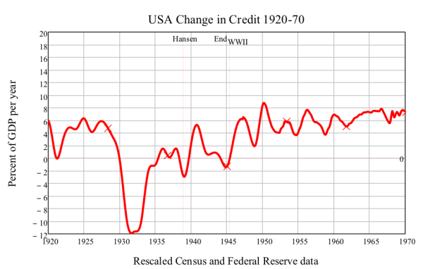
Even more pointedly, unbeknownst to Hansen, a recovery had started just before he proposed the secular stagnation hypothesis (see Figure 5), and for reasons that his supply-side theory did not contemplate: a turnaround in the growth of credit (see Figure 7). The real cause of both the Great Depression itself, and the collapse of the Roosevelt Recession was not “secular stagnation,” but debt-deflation, as rival economist Irving Fisher had asserted in 1933 (Fisher, 1933). During the Roaring Twenties, credit growth averaged 4% of GDP per annum[6] while in the 1930s, it fell to minus 3.4% p.a.[7] The recovery before the Roosevelt recession occurred predominantly because the rate of private sector deleveraging slowed down, and from mid-1935 till the end of 1937, credit growth was actually positive.

However, from 1938 till 1939, the growth of credit declined and turned negative again—possibly in response to the attempt by the Roosevelt administration to return the government budget to surplus—and renewed deleveraging reduced aggregate demand and drove unemployment back up to 20%. From that point on—just before Hansen’s Presidential Address—credit growth resumed, while GDP also boomed thanks to the massive increase in government spending to finance WWII.

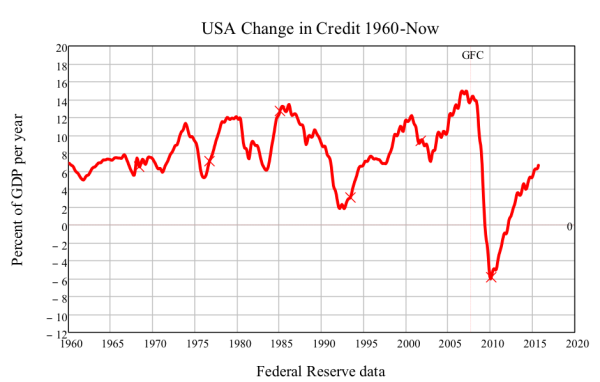
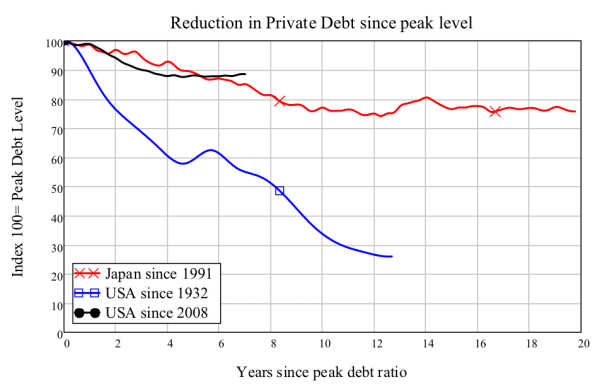
By the end of the War, private debt had fallen to 27% of the peak level reached in 1933 (see Figure 9), and the stage was set for a credit-driven revival in Post-War aggregate demand. From 1945 till 1970, credit expanded at an average 5.7% p.a.—substantially faster than the expansion of credit during the Roaring Twenties. From 1970 until the crisis began in 2008, the expansion in credit averaged 9% of GDP per year (see Figure 8).

Figure 7: Change in private debt from 1920-1960

Figure 8: Change in private debt from 1960-Now

No such sustained credit-driven boom is possible in either Japan or America today, because the deleveraging after their two crises has only slightly reduced private debt levels. Japan’s private debt ratio today is still 75% of the peak level reached in 1996; similarly, America’s private debt level today is 88% of the peak level reached in 2008 (see Figure 9).

Figure 9: Deleveraging as the crucial difference between Golden Age America and today

Why high debt restricts economic growth

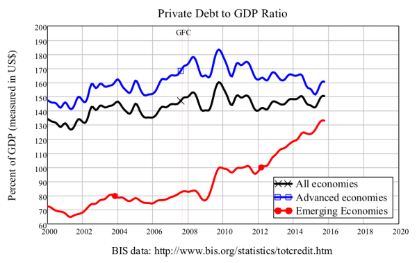
With private debt at today’s levels—an average of 160% of GDP for advanced economies 135% for emerging countries, and 150% for the global economy (see Figure 10)[8]—not only is a sustained credit-driven recovery impossible, but even a slight deceleration in credit growth is sufficient to cause a significant fall in aggregate demand.

Figure 10: The global private debt level peaked in 2010

As I have argued above, the reason that a slowdown in the rate of growth of private debt causes an economic crisis is that this reduces—and often turns negative—a major source of aggregate demand and income. As I explain in the Appendix, it is economically and mathematically valid to treat aggregate demand in a pure private sector economy as the sum of the turnover of existing money, plus the change in debt. The former is crudely measured by nominal GDP; the latter is more accurately measured as the change in debt; and both are dimensioned in currency units per year.

Moreover, the evidence suggests that the higher the debt levels the greater the impact a slowdown in the expansion of credit will have on economic growth.  To illustrate this, let’s make a thought experiment using two hypothetical cases; both cases have the same GDP and debt growth rates, but one has a high level of debt and the other a low level of debt. We consider the impact of a slowdown in the rate of growth of debt from faster than GDP for all but the last year, to zero in the final year. In order to highlight the impact of the debt slowdown alone, we pretend that GDP still continues to grow at the same rate in the final year.

Table 3 illustrates the impact on aggregate demand of a cessation of debt growth in 2017 in an economy where GDP and private debt are growing at the average rates reported for China since 2008—a nominal GDP growth rate of 14% p.a. and private debt growing at 22% p.a.—and where the debt to GDP ratio matches China’s in 2008 and 2016. If private debt simply stops growing in 2017, then even if GDP growth continues at the same 14% p.a. rate in 2017, the growth rate of nominal aggregate demand will fall from +16% to -17% p.a.

Table 3: Aggregate demand illustration with Chinese growth rate & debt ratio data

On the other hand, if we consider an economy with the same GDP and debt growth rates, but a much lower initial debt to GDP ratio of 40% (similar to that of the USA in 1945), then the same phenomenon (a cessation of debt growth while GDP growth continues unaffected) sees the nominal growth rate fall from 15% to 1%—a significant slowdown, but not a crisis.

Table 4: Aggregate demand illustration with Chinese growth rate data and USA 1945 debt ratio

This illustrates the logic behind the empirical pattern uncovered by Richard Vague. Vague found that every major financial crisis since 1850 has involved the private debt to GDP ratio exceeding 150% of GDP, and rising by 17% or more of GDP over a 5-year period prior to the crisis: only when debt is that high does a slowdown in its rate of change cause a serious economic calamity.

The 2007-8 crisis was a global crisis because (a) the collapse in credit growth in the USA alone caused a 7% of global GDP fall in aggregate demand—the change in credit in the USA went from plus 5% of global GDP in 2007 to minus 1.7% of global GDP in 2010; and (b) many other developed nations were in a similar situation, so the decline in credit growth in the rest of the developed world was actually more severe than in the USA (see Figure 3: America’s credit growth went from plus 15 to minus 5 per cent of GDP across the crisis; the average for the advanced economies was from plus 25 to minus 12 per cent).

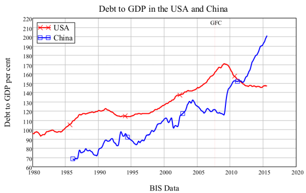
The dilemma the global economy finds itself in now can be explained by the following three realities.  First, almost all leading OECD nations are facing the aftermath of such crises, and have not de-levered sufficiently to allow credit growth to resume.  Second, aggregate private sector debt peaked in 2010 at a level well in excess of the first of Vague’s two criteria for crisis, and while the second is not fulfilled at the global level, credit growth is now stagnant, so that demand from credit growth at the global level has ceased—see Figure 10.  And third, the one major global economy that has not yet experienced such a crisis—China—is, based on its current data, certain to experience one in the near future (see Figure 11).

Figure 11: Debt to GDP ratios in the world’s largest advanced and emerging economies

Conclusion

Koo’s balance-sheet constrained analysis is a sound explanation for Japan’s sustained stagnation, and makes Japan’s situation a foretaste of what the rest of the world will experience now that it has joined Japan in the trap of excessive private debt.  China, the Euro-zone, Japan, and the USA are all private debt constrained.  And thus it is not inappropriate to posit the idea of a “global balance sheet recession.”

The policy implications of this analysis are obvious, if challenging. Firstly, a way must be found to reduce private debt levels drastically, without at the same time triggering the collapse in aggregate demand from such a deleveraging itself. Secondly, the private debt to GDP level must be treated as a crucial macroeconomic indicator, in the way that inflation and unemployment are now. Fortunately, methods to achieve these aims can be devised, but they go against the grain of conventional economic policy.

Private banks are not the only institutions that can create money: so can the government via its Central Bank. Unfortunately, Central Banks in general have not done this in response to the crisis, but have instead created additional Reserve assets for private banks by buying securities from them under the policy of “Quantitative Easing.” This alters the composition of bank assets—and encourages purchases of shares and property, thus inflating asset prices—but does not inject money into the deposit accounts of the private non-bank public, which is what is needed if money is actually to be created and aggregate demand increased.

A shift to what has been described as “People’s QE” could create money by directly crediting household and private non-financial corporation bank accounts.   This same capacity could also reduce private debt if debtors were to be required to pay down their debts, whereas savers—those without bank debt—would receive a cash injection. Many other ancillary policies would be needed, but such a policy would enable private debt to be reduced without reducing aggregate demand. Richard Vague also suggests several mechanisms for private debt reduction which are consistent with current banking practices (Vague, 2014).

The tragedy is that although there are methods by which we could escape the global private debt trap into which we have fallen we are nonetheless prisoners of an economic orthodoxy that will prevent us from employing them… The main barrier here is simply the ignorance of the supposed experts on economics about the nature of money. While mainstream economists continue to spout naïve arguments about money and banking, the politicians who rely upon them for guidance are unlikely to attempt anything other than the poorly targeted and largely ineffective policies that Japan has persisted with for the last quarter century. A global “Lost Decade” is entirely probable.

Appendix 1: Change of debt in aggregate demand and income

Just as it is a truism that “one person’s liability is someone else’s asset”, so is it a truism that “one person’s expenditure is another person’s income.” As I have argued above, the first truism does not allow you to blithely dismiss the role of the change in debt in macroeconomics, as mainstream economists do. The change in debt can only be relegated to a second-order phenomenon in a world in which lending does not alter the liabilities and assets of the banking sector.

A similar observation applies to the second truism: the fact that expenditure is identical to income does not prevent the change in debt in playing a role in both. Expenditure and income are only independent of the change in private debt if the change in debt does not alter the liabilities and assets of the banking sector. There is thus a one-to-one link between the “Loanable Funds” model of lending—in which banks do not originate loans—and the absence of any major macroeconomic impact from lending.

The next three tables illustrate this argument. Consider an economy with a banking sector B and three non-bank sectors S₁, S₂, and S₃, where S₁, S₂, and S₃ also represent the amount of money that the sectors have in their bank accounts. Each sector x spends that balance on sector y at a rate given by the factor t_xy (where this a “time constant” dimensioned in years—see https://en.wikipedia.org/wiki/Time_constant for an explanation if needed). The diagonal cells show expenditure by each sector on the others; the off-diagonal cells show the receipt of that expenditure by the other sectors, which is their income. Each row necessarily sums to zero, while each column shows net income for each sector (which can be positive or negative). The negative sum of the diagonal cells is aggregate expenditure (AE); the sum of the off-diagonal cells is aggregate income (AY); and the two are necessarily equal in all 3 tables.

Table 5 shows what happens when no borrowing is possible: all demand and income is generated out of the turnover of the existing money stock, and of course change in debt plays no role (for simplicity, no activity is shown for the banking sector).

Table 5: No lending possible

Table 6 shows the model of “Loanable Funds”, in which banks arrange but do not originate loans (for the sake of simplicity, both bank fees and expenditure by banks are ignored here). In this instance, sector 1 borrows from sector 2 to spend on sector 3, and sector 2 makes these funds available by not spending them on sector 3 itself (more complicated situations could be shown without changing the final conclusion).

Table 6: Loanable Funds—Banks do not originate loans

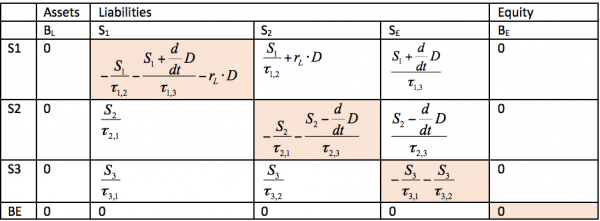
Table 7 shows the real-world situation of “Endogenous Money”, in which banks originate loans and simultaneously create money—which in this example is spent by sector 1 to purchase the output of sector 3. Sector 1’s borrowing creates a flow of new debt for the banking sector, and this is spent by sector 1 on the output of sector 3.

Table 7:Endogenous Money—Banks originate loans

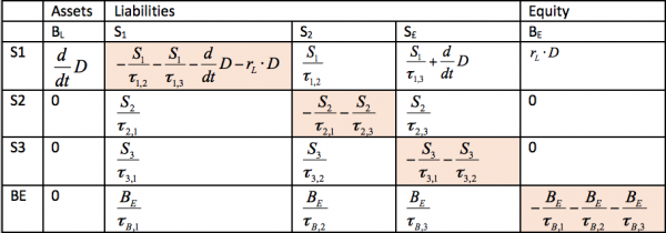
In this real-world case, there is no offsetting reduction in spending by any other sector, and the full amount of the change in debt turns up as a component of both aggregate expenditure and aggregate income:

The macroeconomic interpretation of this outcome—that change in debt forms part of both aggregate demand and aggregate income—is that aggregate demand has 2 key components: demand from the circulation of existing money, plus demand from the creation of new money by the banking sector (the third component is gross financial transactions).

Since the vast majority of credit money today is created to finance purchases of assets rather than goods and services, the proper recognition of the role of banking in macroeconomics also requires the integration of macroeconomics and finance. Rather than aggregate demand being identical to aggregate income, the proper relationship is that aggregate demand is identical to the sum of aggregate income plus realized capital gains.

Appendix 2: Long-term debt series for the USA

Since 1952, the Federal Reserve has published detailed quarterly data on US private debt levels in its “Flow of Funds” (now renamed the “Financial Accounts of the United States”—see http://www.federalreserve.gov/releases/z1/). Before then, the Bureau of the Census published two overlapping series on debt of the nonfinancial private sector (from 1916 till 1970) in the publication Historical Statistics of the United States: Colonial Times to 1970 (http://www2.census.gov/prod2/statcomp/documents/CT1970p1-01.pdf), and selected assets of banks (from 1834 until 1945) in the publication Historical Statistics of the United States 1789-1945 (http://www2.census.gov/prod2/statcomp/documents/HistoricalStatisticsoftheUnitedStates1789-1945.pdf). Though the three series give substantially different aggregate levels for private debt, the correlations between changes in the three series are quite strong where they overlap. The correlation of the annual change in the bank loan data with the annual change in nonfinancial sector debt from 1916 till 1945 is 0.78, while the correlation of the Census data for annual change in nonfinancial sector debt with the “Flow of Funds” data for 1952 till 1970 is 0.56.

I therefore rescaled the Census data to coincide with the Federal Reserve data to produce a pseudo-Flow of Funds time series for private debt from 1834 till today, as shown in Figure 12. This data series was used to make comparisons between the growth of credit during the Roaring Twenties and the Great Depression, and the Post-WWII period.

 Figure 12: The long term history of US private debt

This imputed data set supports an assertion I have made in the body of this paper, that the world has now reached a level of private debt that is unprecedented in the history of capitalism. No comparable long-term private debt data series exists for any other nation, but it is, I believe, highly unlikely that any previous peak in private debt exceeds the one that we are experiencing now.

References

BELL, S. 1998. The Hierarchy of Money. Levy Economics Institute, The, Economics Working Paper Archive.

BERNANKE, B. S. 2000. Essays on the Great Depression, Princeton, Princeton University Press.

FIEBIGER, B. 2012. Modern Money Theory And The ‘Real-World’ Accounting Of 1-1<0: The U.S. Treasury Does Not Spend As Per A Bank. PERI Political Economy Research Institute. Amherst: University of Massachusetts.

FIEBIGER, B. 2014. Bank credit, financial intermediation and the distribution of national income all matter to macroeconomics. Review of Keynesian Economics 2, 292-311.

FISHER, I. 1932. Booms and Depressions: Some First Principles, New York, Adelphi.

FISHER, I. 1933. The Debt-Deflation Theory of Great Depressions. Econometrica, 1, 337-357.

FONTANA, G. & REALFONZO, R. (eds.) 2005. The Monetary Theory of Production: Tradition and Perspectives, Basingstoke: Palgrave Macmillan.

GRAZIANI, A. 1989. The Theory of the Monetary Circuit. Thames Papers in Political Economy, Spring, 1-26.

HANSEN, A. 1939. Economic Progress and Declining Population Growth. American Economic Review, 29, 1-15.

KEEN, S. 2011. Debunking economics: The naked emperor dethroned?, London, Zed Books.

KEEN, S. 2014. Endogenous money and effective demand. Review of Keynesian Economics, 2, 271–291.

KEEN, S. 2015. The Macroeconomics of Endogenous Money: Response to Fiebiger, Palley & Lavoie. Review of Keynesian Economics, forthcoming 3.

KOO, R. 2009. The Holy Grail of Macroeconomics: Lessons from Japan’s Great Recession, Wiley.

KOO, R. 2011. The world in balance sheet recession: causes, cure, and politics Real-World Economics Review, 58, 19-37.

KOO, R. C. 2003. Japan’s Lesson for America. International Economy, 17, 62.

KOO, R. C. 2014. It Is Private, Not Public Finances that Are Out of Whack. German Economic Review, 15, 166-190.

KRUGMAN, P. 2012. End this Depression Now!, New York, W.W. Norton.

KRUGMAN, P. 2013. Abenomics and Interest Rates: A Finger Exercise (Wonkish) [Online]. New York: New York Times. Available: http://krugman.blogs.nytimes.com/2013/06/10/abenomics-and-interest-rates-a-finger-exercise-wonkish/.

LAVOIE, M. 2014. A comment on ‘Endogenous money and effective demand’: a revolution or a step backwards? Review of Keynesian Economics, 2, 321 – 332.

MCLEAY, M., RADIA, A. & THOMAS, R. 2014. Money creation in the modern economy. Bank of England Quarterly Bulletin, 2014 Q1, 14-27.

MINSKY, H. P. 1980. Capitalist Financial Processes and the Instability of Capitalism. Journal of Economic Issues, 14, 505-523.

MOORE, B. J. 1979. The Endogenous Money Stock. Journal of Post Keynesian Economics, 2, 49-70.

SUMMERS, L. 2014. Reflections on the ‘New Secular Stagnation Hypothesis’. In: TEULINGS, C. & BALDWIN, R. (eds.) Secular stagnation: Facts, causes, and cures. London.

VAGUE, R. 2014. The Next Economic Disaster: Why It’s Coming and How to Avoid It, Pennsylvania, University of Pennsylvania Press.

VOUTSINAS, K. & WERNER, R. A. 2011. Credit supply and corporate capital structure: Evidence from Japan. International Review of Financial Analysis, 20, 320-334.

WERNER, R. A. 2002. Monetary Policy Implementation in Japan: What They Say versus What They Do. Asian Economic Journal, 16, 111-151.

WRAY, L. R. 1989. The Endogenous Theory of Money. Ph.D., Washington University.